Hello again!

In this post I want to cover how to create a hierarchy of the layers described in my previous posts, as well as how to use it for reinforcement learning!

The previous posts are available here:

https://cireneikual.wordpress.com/2014/12/21/continuous-hierarchical-temporal-memory-chtm-update/

https://cireneikual.wordpress.com/2014/12/24/continuous-hierarchical-temporal-memory-temporal-inference/

Forming Hierarchical Predictions

Continuing from where I left off, we now have layers that produce sparse distributed representations of their input and then predict that input one step ahead of time.

Adding a hierarchy allows predictions to traverse longer distances along the layers. The basic idea is this: Create a hierarchy where the higher layers are typically smaller than lower ones. Then form SDRs in a bottom-up order, such that each layer forms a SDR of the layer below it.

In the bottom-pass we only form SDRs, we don’t form predictions yet. This happens in the next top-down pass.

To get less local predictions at lower layers, we can then perform a top-down pass where each layer gets an additional “temporary” context cell whose state is equivalent to the prediction of the next higher layer at the same coordinates. This temporary cell is treated like all other cells, and the other cells must maintain connections to it that are learned as usual.

In summary: We ascend the hierarchy by forming SDRs, and then descend again and form predictions where each layer gets additional context from the previous layer.

Reinforcement Learning, a Quick Summary

In reinforcement learning, the AI or “agent” seeks to maximize a reward signal. This is similar to how animals and humans learn. Since HTM is inspired by biology, it seems natural to try to use HTM for reinforcement learning as well.

Here we will use temporal difference (TD) learning. More specifically, we will use Q learning. As a result we must somehow maintain a Q function that represents the “quality” or “desirability” of each state. If we can somehow use HTM as a function approximator, we can simply store and update Q values using that.

Recall the Q learning equation (I “stole” this image from wikipedia):

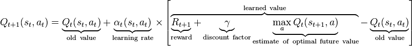
The portion of the equation after and including the learning rate is the temporal difference error, which is usually backpropagated as an error value in standard neural networks to update the Q function.

Function Approximation with HTM

As stated above, we need a function approximator to model the Q function. HTM isn’t well know for use in function approximation, but there is a way of doing so, and it is quite effective! Not only do we get to approximate the Q value for each observable state, but it is trivial to also include the context available from the context cells. So, we can essentially reproduce the results of standard recurrent neural network architectures like LSTM, and can do so without the problem of forgetting previously learned values!

This sounds great and all, but how do we do it?

The secret is as follows: Make another standard neural network pass through all cells/columns and use standard backpropagation techniques to update it.

It is possible to pass just through columns if you don’t care about contextual information, like so:

However, for the most effective reinforcement learning we want each cell to connect to all cells in the previous layer within a receptive radius so that we also have contextual information. So a single column is connected fully to a column of the previous layer like so:

For those of you accustomed to deep learning, you may be wondering why the HTM portion even exists if it only provides pathways for a standard network. You may also be wondering how to update such a monstrosity with backpropagation.

Recall that a layer of HTM is very sparse, both in terms of column and cell states. So, consider that we only activate and train portions of this standard network only if they pass through an active cell/column. Suddenly, training becomes far more manageable, since only very small amounts of the network are active at a time. It also becomes incredibly efficient, since we can effectively ignore cells/columns and their sub-network when they have a very small or equal to 0 state value.

Some of you may notice that this is astoundingly similar to the dropout technique used in standard neural networks. Indeed it is, and also comes with the nice regularization benefits.

Here is an example of a cross-section showing a SDR-routed subnetwork:

Furthermore, this has the benefit of only activating certain subnetworks in certain situations while taking context into account!

So, we can train this as our Q function now using standard backpropagation! The only difference is that in the forward pass we multiply the output by the HTM cell/column state, and in the backward pass the derivative changes a bit as a result.

Action Generation

The Q function is now done, but then how do we get actions from it now?

So here it gets kind of weird. There are several alternative solutions to getting actions from a Q function, but I found that simply backpropagating very high Q values all the way to the inputs and then moving those inputs along the error results in an efficient hierarchical action selection scheme.

So when defining the input to the system (input to the bottom-most layer), we need at least 2 different kinds of inputs: State, and action. Here is an example of how they may be organized:

Where green values are state values and blue values are action values.

The scenario above could for instance be an image presented as a state and 2 action outputs.

So what we do is backpropagate a high positive error value all the way to the action inputs, and the move the action inputs along the error to get an action with a higher Q value.

From there, we can apply some exploration (random perturbation), and ta da, we now have actions!

The number of iterations necessary to produce the actions needs to be at least 1, but it doesn’t need to be much larger than 1 either. Since the action is also presented as input to the HTM, we can use the HTM’s predictions to get a starting point for the action backpropagation process. So we can remember “where we left off” and continue the action search from there the next time we enter the same (or similar) state.

Conclusion

I am currently still in the process of fine-tuning these algorithms (the difficulty is in the details), but what I have presented is the overarching idea. I hope it made sense!

If you would like to follow the development of my GPU implementation of this theory, here is the GitHub repository: https://github.com/222464/ContinuousHTMGPU

Have any ideas for improvements to the system? Let me know in the comments!