My Attempt at Outperforming Deepmind’s Atari Results – UPDATE 10

Hello again!

I said in the last post that I would open-source my continuous HTM GPU implementation. Well, here it is! Sorry for the delay! Link: https://github.com/222464/ContinuousHTMGPU

I did a rough performance test on GPU HTM, and I was able to simulate a region with 16384 columns, 65536 cells, 1.3 million column connections and 21 million lateral connections at 80 iterations per second. I don’t know if this is a lot or not, but keep in mind that I have not yet optimized it. My GPU is a Radeon HD5970.

I have been working on my newest version of HTM-RL. The old version was able to solve the pole balancing and mountain car problems quite easily, but had difficulties as soon as one started adding more regions to the HTM. As new regions were added, the HTM would get increasingly stable. However, it gets so stable that one cannot perceive subtle changes in the input from the sparse distributed representation of the topmost region.

So previously, HTMRL could only learn off of very general concepts that don’t change very rapidly (when more than one region is used). So, it could for instance identify where the most enemies in space invaders were located, but it could not distinguish them individually.

I have come up with a new method that will allow it to use information at all levels of the hierarchy. It is a form of hierarchical reinforcement learning.

The idea is as follows: Have each HTM region represent both the state and the last action taken. Then, for each level of the hierarchy, use a function approximator that maps the column outputs to a Q value. Starting at the topmost level in the hierarchy, use a form of gradient descent on the “action” columns to optimize the Q value (make it as large as possible). This becomes the region’s suggested action. From there, descend down the hierarchy, and again optimize the Q values. But, before the optimization takes place, incorporate the next higher layer’s suggested action into the region’s action output (using a weighted average, for instance).

This way we essentially start with the most general, high-level description of the action, and then perturb it into a more and more fine-grained action as we descend down the hierarchy, based on the Q values.

I sort of doubt the biological plausibility of this approach. But I do think it will work (at all). As long as it ends up working, I don’t care about the biological plausibility that much 🙂

Here is a Blender render I made that shows the structure of the function approximator that is attached to a single HTM region. Please excuse my poor modeling skills!

Key:

  • Red – HTM cells
  • Blue – hidden layer (can be convolutional)
  • Green – output layer (linear)

htmrender

By the next update I want to have HTMRL up and running. Let’s see if I can make it!

Until next time!

My Attempt at Outperforming Deepmind’s Atari Results – UPDATE 9

Greetings!

The past 3 days I have spent on writing a fast GPU spatial and temporal pooler. It works! Unlike Numenta’s HTM, it both operates in the continuous domain and is much, much simpler. I don’t think I sacrificed any functionality by converting the discrete logic of the original into continuous formulas.

I sort of just made up formulas as I went, until it gave me the desired result. Not very rigorous, but it got the job done in the end regardless.

So, I would like to now describe the formulas that I came up with. Hopefully someone finds it useful besides myself. Continuous HTM is not well researched, if at all.

I will assume that you know how the original HTM works to some extent. For instance, what the spatial and temporal poolers  are supposed to do.

I am not going to use proper indexing (e.g. wij as opposed to simply w) for formulas, I will rather describe in words how the operation is performed given the indexless formula. This is not supposed to be a paper, just a way of giving a rough idea of how the continuous spatial and temporal poolers work.

Continuous Spatial Pooler

The continuous spatial pooler consists of 2 2D buffers of floats, the activation buffer and the column output buffer.

The activation buffer receives input from another 2D buffer of floats, the input buffer. It has connections to a subregion of the input buffer for each element of the activation buffer. These subregions are positioned such that the normalized coordinates of the positions in both the input and activation buffers are the same.

One can then perform a weighted convolution of the input buffer. For each element in the activation buffer, compute:

formula1

Where a is the activation value, w is the weight of the connection, and in is the input corresponding to the connection. The activation value is stored in the activation buffer.

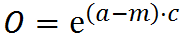
Once all activations have been computed, then comes the inhibition step. In this step, one reads the activation values surrounding the current element within a predefined radius, and finds the maximum. One then deactivates the current element according to how close it is to the maximum. So, something like this:

formula2

Where O is the output to be stored in the column output buffer, is the activation of this element, m is the maximum activation across all elements in the inhibition radius, and c is a constant “intensity” factor.

This is the output of the spatial pooler. However, we are not done with it yet. We need to update the weights to learn unique sparse representations of the input. I used Oja’s rule for this:

From wikipedia:

Oja’s rule defines the change in presynaptic weights w given the output response y of a neuron to its inputs x to be

\,\Delta \mathbf{w} ~ = ~ \mathbf{w}_{n+1}-\mathbf{w}_{n} ~ = ~ \eta \, y_{n} (\mathbf{x}_{n} - y_{n}\mathbf{w}_{n}),

So, for each weight, we want to perform a hebbian-style learning rule. Oja’s rule is a version of the Hebbian rule that does not increase without bounds.

Temporal Pooler

Once we have the outputs of all of the elements of the column output buffer, it is time to compute the outputs of the cells within each column. Cells are represented by 2 3D buffers: The cell state buffer and the cell prediction buffer. The former contains the cell’s outputs, and the latter contains future predictions made by cells. We also have an additional column predictions buffer, which is 2D, and represents the predictions the cells gave to a column.

We first use a “soft” winner-takes-all scheme (so more like “winner takes most”) in order to give a higher output to cells which were previously predicted most accurately. This helps form a context for a column. The cells indicate which predictions activated this column into the predictive state, allowing future context-sensitive predictions to occur.

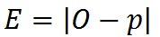
So, we first compute the prediction errors for each cell. This is simply the absolute value of the difference between the current column output O, and the cell predictions from the previous frame:

formula3

While doing so, we keep track of the smallest error, which we will call x.

The output (state) of a cell is then:

formula4

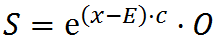
where c is again an “intensity” constant (doesn’t need to be equal to the previously mentioned c, it’s a different constant).

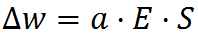
Once we have computed all cell activations, it is time to update the weights a cell has to all other cells in a radius. These are called lateral connections. They are updated according to their cell’s prediction error as well as the state of the source cell from the previous time step:

formula5

Once we have updated the weights, it is time to make our prediction of the next frame’s input. This is a function of the summation of the weights multiplied by their respective cells’ states:

formula6

where w is in this case the cell lateral weights, S is the cell state to which the weight corresponds, and is again an “intensity” constant, which can be different from the previously mentioned c‘s.

Finally, we create a column prediction from the cell predictions. This is simply the highest prediction in the column:

formula7

where P is the column’s prediction.
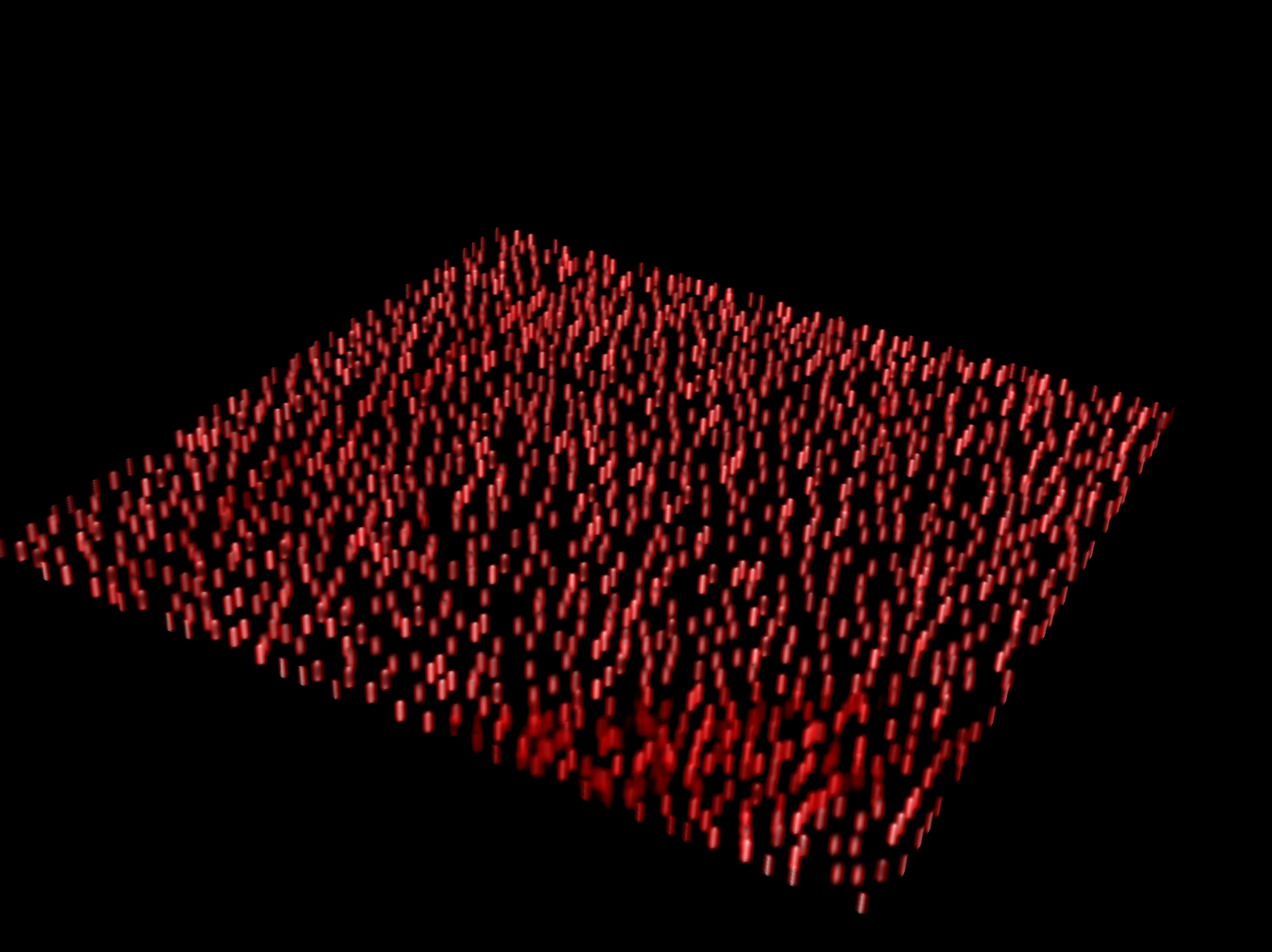
The Result

I would make a video, but I fear it would be too difficult to explain what it means. So instead, I will release a demo program along with source code within the next few days. Until then, you will have to take my word for it that it indeed works! I will edit this post to contain the link as soon as it is available.

Edit: The link: https://github.com/222464/ContinuousHTMGPU

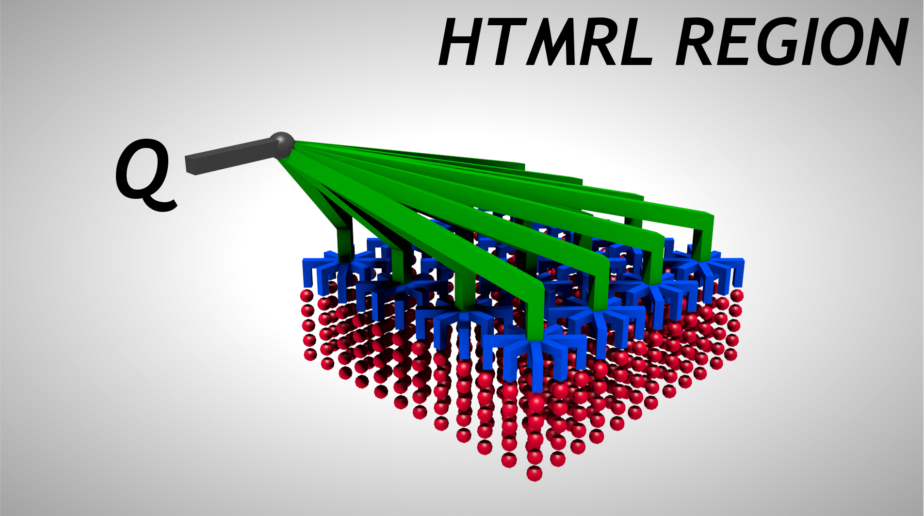
How is this useful for outperforming Deepmind?

I have a plan on how to elegantly combine this continuous HTM with reinforcement learning, based on concepts discussed in my previous post. I will explain it in the next post, since this one has become quite long already.

See you next time!

My Attempt at Outperforming Deepmind’s Atari Results – UPDATE 8

Hello again!

I recently found an interesting paper (http://www.plosone.org/article/info%3Adoi%2F10.1371%2Fjournal.pone.0029264). It describes a method for applying MPF (a superset of HTM, Memory Prediction Frameworks) to reinforcement learning, and I really like the idea behind it so far.

From what I gather, the idea is to do an upward pass on the MPF to form increasingly invariant and abstracted forms of the current and past inputs. One then descends down again and combines information from the upper levels with the more fine-grained information at the lower levels. While doing this, one can perturb predictions such that the system is more likely to predict inputs (consisting of state and action) that lead to higher rewards.

The authors actually mentioned that they also wanted to use it for game playing, which is my goal. Since then I have been very excited at the prospect of using MPF and MPF alone to do the reinforcement learning, and have started extending my existing GPU-HTM to include temporal pooling as well as the backwards pass and action-generating perturbations.

Possible benefits of this approach over using MPF solely as a feature extractor:

  • Features at each level in the MPF hierarchy can be used, and combined with features from previous higher layers on a backwards pass to add additional context to actions.
  • No need for experience replay, which is slow and inelegant – MPF is designed to work online from the beginning.
  • Can be run easily on the GPU, using images (textures) to store weights, activations.
  • Partial observability is easier to handle.

Possible negatives of this approach:

  • Less material to work with – less papers. If something goes wrong, I am unlikely to find too much help.
  • Input encoding may be difficult. However, since my version of HTM operates using continuous cell and column states, this might not be as difficult as it first seems.

I have already written a GPU temporal pooler with one-step prediction, which should be sufficient for now. As with my spatial pooler, it operates on continuous cell/column states, unlike Numenta’s HTM.

I leave you with an image of the cells in an HTM region responding to a test image (rendered with VolView):

htmcellsimage

Until next time!

My Attempt at Outperforming Deepmind’s Atari Results – UPDATE 7

Hello again!

It’s been a couple of days, so I would like to show what I have been working on.

I now have image-to-features system, one fully functional and another that was functional but is receiving an overhaul. The former is an implementation of HTM’s spatial pooling in OpenCL. Unlike the CPU version though, this version works with continuous values. It forms sparse distributed representations of the input, but leaves out the temporal pooling portion of the fully HTM algorithm. The temporal pooling is significantly more complicated than the spatial pooling and not nearly as GPU-friendly, so I decided to just do spatial pooling for now and let the reinforcement learner take care of partial observability.

The second system is a convolutional stacked autoencoder. It runs online, and was rather difficult to parallelize due to the need for a summation of all of the gradients for each position of the filter in the receptive field. To parallelize the summation, I made a large reusable buffer that stores all the gradient values for all the convolution positions, and then did an additive downsampling. This adds 4 sub-gradients at a time (a 2×2 square) in parallel. I originally had max-pooling, but since I do not want translational invariance I removed it again.

Here is an example of a set of unique features derived from a screen of “space invaders” using the GPU-HTM:

featuresHTM


Here is an example of the convolutional autoencoder (GPU-CAE) representing the number 2:

cae

The code is not part of the main repository yet, but I will soon upload the modified ALE along with the new code.

That’s it for this update!

See you next time!

My Attempt at Outperforming Deepmind’s Atari Results – UPDATE 6

Hi!

Another update!

I have been working on the image-to-features system. Deepmind did not have a separate feature extractor and reinforcement learner. They used a convolutional neural network to predict Q values for discrete actions. While I have both a discrete and continuous version of HTMRL, I really want to focus on the continuous version since it can be applied to more problems in the future. However, the way I am currently obtaining a continuous policy from a Q function makes it far more efficient to separate the structures for image feature extraction and reinforcement learning instead of combining them.

I fixed several large bugs in my HTM implementation that were causing it to predict poorly. In case this HTM stuff doesn’t work out though, I tested a convolutional restricted boltzmann machine network on the pole balancing problem. In case I do end up pursuing this route instead of HTM, I would need to handle partial observability in the reinforcement learning portion of the algorithm.

In HTMRL, partial observability is handled by the HTM itself: It produces novel patterns that combine both current state and predicted future state. A problem I am currently having with it though is that unless I make the receptive field of the HTM columns very small, it will not perceive small changes in the image. It will instead just ignore them. It is possible to remedy this by adding more and more columns, but this drastically slows down the algorithm. Therefore I am currently experimenting with different parameters and topologies to find what works best. If I absolutely cannot get it to work, I still have that Conv-RBM.

In case I do end up using Conv-RBM instead, I would need to handle partial observability differently. Fortunately though, I was already able to solve problems such as the T-maze problem by simply feeding the hidden units used by the free-energy based reinforcement learner back to the visible units. To be honest, I didn’t expect such a simple solution to work, but it worked. So, unlike Deepmind’s algorithm, I now can learn “infinitely” long-term dependencies (theoretically anyways). Deepmind used a fixed-size history window as far as a know, which both increases the complexity of the resulting MDP and cannot account for long-term dependencies that require knowledge beyond this time window.

In case you missed it, the free-energy based reinforcement learner (FERL) I use for the continuous version of HTMRL is derived from this: http://www.ncbi.nlm.nih.gov/pmc/articles/PMC3584292/. I modified it heavily to perform both continuous actions and handle partial observability.

So, to summarize: HTM, or Conv-RBM + recurrent hidden nodes in the reinforcement learner portion. I will probably end up doing both 😉

For those just seeing this for the first time, the source code for this is available here, under the directories “htmrl” and “convrl”: https://github.com/222464/AILib It uses the CMake build system.

Until next time!

My Attempt at Outperforming Deepmind’s Atari Results – UPDATE 5

Hey everybody!

Another update!

The reinforcement learning portion is done, so now I turn my attention to the image recognition portion so that I may scale up better to the ALE. I originally tried to go immediately to the ALE, but it takes so long to find out whether or not what you did is working so instead I decided to stay with pole balancing. However, instead of feeding values such as position and velocities of the cart directly to the HTM bottom-most region, I am now using an encoding of the image of the experiment. This provides me with an intermediate step on the path to scaling up to the ALE.

At this point, I could dump the HTM stuff and just do ConvNets, but that feels like a cop out. I have found an interesting paper that compares CLA (HTM) to the state of the art, and they showed that it indeed outperforms things like convolutional neural networks (they used LeNet), mostly due to the time signal, on tasks where sequences of information are presented. I have such a task. So, I will continue working on my HTM implementation and improving it. I am currently in the process of reading that paper (available here:http://bias.csr.unibo.it/maltoni/HTM_TR_v1.0.pdf) to see how they were able to adapt it for classification (from which I can adapt it to function approximation).

EDIT: Upon further examination, the paper’s validity appears questionable. The “HTM” they use is also very different from Numenta’s HTM (the one I am using).

I am still not quite certain if I am encoding the greyscale images properly for the HTM, right now the regions are way too stable. The previously mentioned paper talks of feedback signals from higher regions in the hierarchy that allow for adaptation of lower levels with the context gathered from the higher levels. My current HTM model does not have this, so I am very interested in seeing how that affects things for reinforcement learning.

Right after this post, I will continue reading the paper, and start coding a new HTM model. Besides incorporating any improvements I can gather from the paper, I am moving everything to the GPU using OpenCL. I used to be mainly a graphics developer, so this shouldn’t take too long to do 🙂

For those just seeing this for the first time, the source code for this is available here, under the directory “htmrl”:https://github.com/222464/AILib It uses the CMake build system.

That’s it for this update, until next time!

My Attempt at Outperforming Deepmind’s Atari Results – UPDATE 4

Hello again!

As I stated in my previous posts, the precision of the function approximation remains a problem. However, I have found that using SARSA instead of Q learning (on-policy instead of off-policy) mitigates the problem a lot since it is no longer bootstrapping on the largest potential value (subject to overestimation) but rather the potential value of the selected action.

Due to this improvement, I decided to move back to feed-forward neural networks with RMS training. The RBF networks train much faster, but they seem to forget things faster (things not part of the replay chain). I assume this is due to the on-line supervised learning that occurs, which can destroy previously learned information quite easily in favor of better matching new information.

I now have HTMRL performing both pole balancing and the mountain car problem with very little training time. It figures both of them out in under a minute usually.

I started scaling up to the Arcade Learning Environment, and did some short test runs. I also did a lot of optimization, since I want it to run in real-time (Deepmind’s algorithm was not in real-time as far as I know, and took more than just one standard desktop PC). I have not yet trained it enough to get decent results (5 minutes is not much), but I will probably try an overnight run soon.

For the continuous action edition of the algorithm, I experimented with free-energy based reinforcement learning. It learns a value function as usual, but it can easily derive a continuous policy from the value function. I started implementing replay updates for this as well.

Here is a short video of the system learning the mountain car problem:

For those just seeing this for the first time, the source code for this is available here, under the directory “htmrl”:https://github.com/222464/AILib It uses the CMake build system.

It’s getting there!

See you next time!

My Attempt at Outperforming Deepmind’s Atari Results – UPDATE 3

Greetings!

Update time!

As in my previous update, I am still having problems with the function approximation not being exact enough. I found some papers describing how using function approximation with Q learning can lead to over-estimation of the Q values. Indeed, I noticed that when I changed the reward function, it would typically either not decay from the highest Q values or do so very slowly. To remedy this, I tried force-decaying Q values over time upon state visitation, but this didn’t really help.

So after that, I attempted getting a more exact function approximation. I tried using radial basis function networks instead of the plain old feed-forward neural networks. Results here are promising, I immediately noticed a reduction in temporal difference error values (which would indicate it predicting properly more often). As far as I know, radial basis function networks often have their prototypes/centers pre-trained using K-means clustering. However, since I am developing an entirely online algorithm, I had to adapt it to work continuously. To do so, I implemented a sort of competitive unsupervised learning strategy that mirrors an online form of K-means clustering. I tested it on some benchmark supervised learning tasks, and I got much faster learning rates than with feed-forward neural networks (I was able to consistently learn an XOR in 30 updates).

I also began taking a deeper look into policy gradient methods, since these are supposedly less affected by inaccuracies in function approximation. I may end up using a natural policy gradient method.

On the HTM front, I only did some tuning of parameters. I am actually quite pleasantly surprised by how well it works, with all the scrutiny it is under I expected worse. It produces stable patterns (same state gives same pattern, with some generalization allowed) for my function approximators. We will soon see how well it scales up though 😉

Here is a video of it predicting the motion of a box. It is a bit old, I made it when I first got it working, but I thought I should share it anyways. The left side is input, the right side is output. When the left is blue, it is the “true” input, when it is red, it is the distributed representation.

That’s it for this update, progress is being made, slowly but surely!

Here is a link to the source code. The repository containts many agents, the one these posts are focusing on is called HTMRL and can be found in the directory of the same name! https://github.com/222464/AILib

My Attempt at Outperforming Deepmind’s Atari Results – UPDATE 2

Hello again!

I am now (almost) satisfied with the performance of the system on pole balancing. The main issue I am having right now is with the function approximators for the actor/critic. They are slow and lack enough precision. Fortunately though, the switch to advantage(lambda) learning helped remedy the inaccuracy in the function approximation to some extent. I need massive Tau values to get decent performance, so increasing the accuracy of the function approximators is a top priority.

Aside from that, I worked on the generalization capabilities of the function approximators. I added regularization and early stopping. I also started using a combination of epsilon-greedy and softmax action selection.

I also experimented with using separate function approximators for each action (for the discrete action version). The intuition behind this is that this will reduce error interference and make it easier to learn the larger differences in outputs that result from advantage learning.

I added plotting capabilities using sfml-plot, allowing me to better observe what effects my changes have.

Here is an image of the pole balancing experiment with plotting:

Until next time!