Hello!
When working on HTFE, I spend a lot of time dealing with how one properly creates SDRs (Sparse Distributed Representations, aka sparse codes) for inputs. I have recently created a semi-new method of generating sparse codes in a very fast manner that, to my knowledge, is biologically plausible.
What are SDRs/sparse codes? SDRs are representations of data where most entries are 0 (sparse). The main reason I find this interesting in particular is how it can be used for efficient feature extraction as well as reducing or eliminating catastrophic interference in reinforcement learning. SDRs are also the way the brain stores information. SDR receptive fields tend to exhibit Gabor-wavelet-like behavior like those found experimentally in animals.
So, how do we go about creating our own SDR learning algorithms? By searching the web, you will find several algorithms which produce similar results. However, many of them are not very biologically plausible or are difficult to reproduce. So, I present an algorithm I came up with after researching this topic for a while.
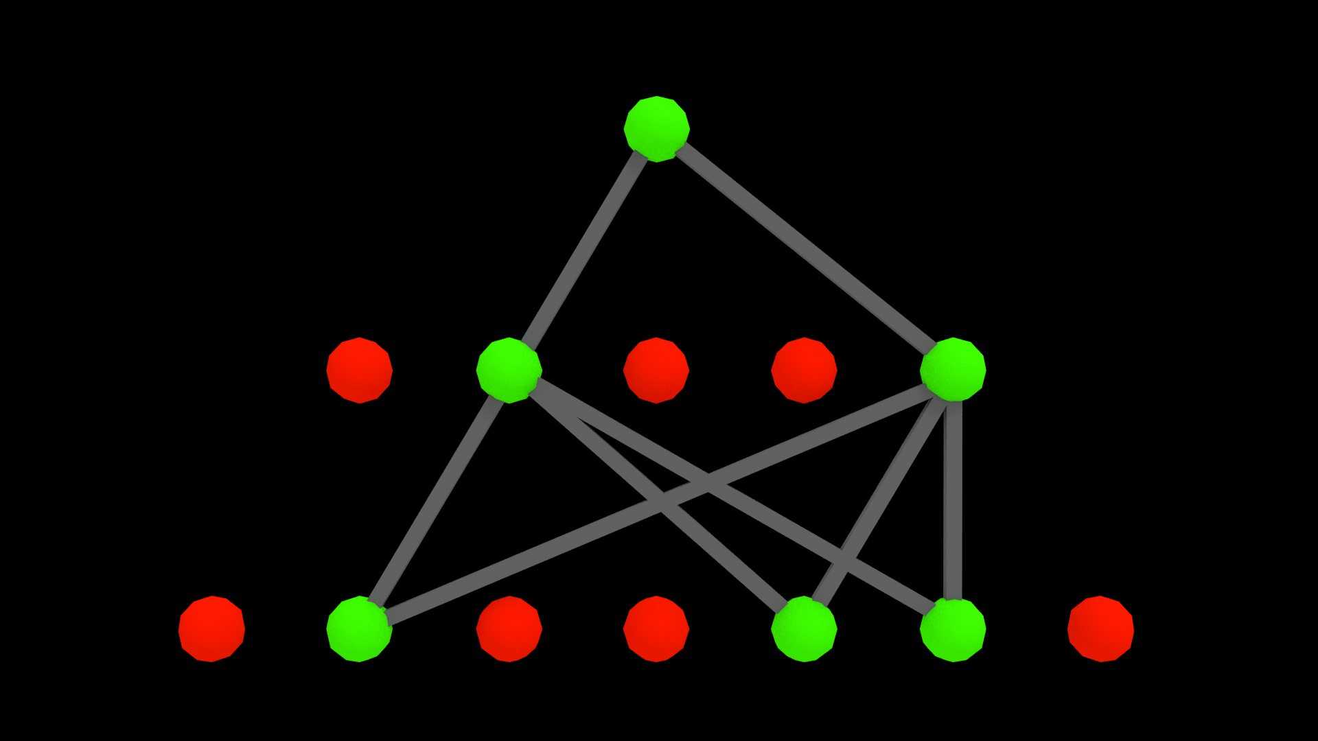
The algorithm consists of a population of nodes which fire when their input is similar to their receptive field. Then, to induce sparsity, these nodes inhibit each other through learned lateral connections. This means that the more often two nodes fire together, the stronger their inhibitory links get. This results in a separation of nodes that respond to similar inputs (decorrelation).
I will try to approach this tutorial from a programming perspective, as I feel it makes it easier to understand what is going on. I will use Python with numpy, as it is relatively easy to understand.
Let’s start by defining some data structures:
self.weights = np.random.rand(sdrSize, numInputs) * (maxWeight - minWeight) + minWeight
self.biases = np.random.rand(sdrSize) * (maxWeight - minWeight) + minWeight
self.activations = np.zeros(sdrSize)
self.inhibition = np.zeros((sdrSize, sdrSize))
Here, weights represents the receptive field. It is a matrix where each row represents a node, and each column represents its weights. The biases act as a sort of threshold weight, it is an array the size of the number of nodes. Activations is also an array the size of the number of nodes, representing the firings of the nodes before inhibition. Finally, inhibition is a matrix of weights that represents the inhibitory connections between nodes (where rows are the current node and columns are the surrounding nodes).
In the above code snippet, the weights and biases are initialized randomly and everything else is set to zero.
To obtain the SDR from these parameters, we do the following:
sums = np.dot(self.weights, inputs.T) + self.biases

self.activations = np.maximum(0.0, sums)

sdr = self.activations - np.dot(self.inhibition, self.activations)

for i in range(0, self.activations.size):
    if sdr[i] > 0.0:
        sdr[i] = 1.0
    else:
        sdr[i] = 0.0
First off, let me say I am not a master Python coder 🙂 Also, I do realize that this code is quite inefficient. But it should work for explanatory purposes.
So, we start by computing sums, which is the integration of each node’s inputs. Then, we apply the activation function to get activations, in this case a simply linear rectifier (max(0, value)).
From there, we get our SDR by inhibiting the activations using the inhibition weights, and then setting each SDR entry to be either 0 or 1.
This completes the SDR generation step. To actually learn proper SDRs, we need to add some additional code:
recon = np.dot(self.weights.T, sdr.T)

error = inputs - recon

for i in range(0, self.weights.shape[0]):
    lscf = sparsity - sdr[i]

    self.weights[i] += alpha * sdr[i] * error

    self.biases[i] += gamma * lscf

    self.inhibition[i] += beta * lscf * self.activations[i] * self.activations

    self.inhibition[i] = np.maximum(0.0, self.inhibition[i])

    self.inhibition[i][i] = 0.0
Here, alpha, beta, and gamma are learning rates.
We start by getting a reconstruction of the SDR. This is basically the information the system “thinks” it is seeing. What we want to do is get the reconstruction to match the actual input as closely as possible, while forming unique SDRs for unique inputs.
Once we have the reconstruction, we proceed to find the error between the inputs and the reconstruction. Then, we go through each node, and first determine the lscf (lifetime sparsity correction factor). This is a measurement of how close the SDR is to the target sparsity.
The weights are then updated through a simple Hebbian learning rule in a way that reduces reconstruction error. The biases are then updated based only on the lscf, since the biases control the relative sparsity of the node.
Finally, the inhibition weights are updated through another Hebbian-like learning rule. This time, it is a measurement of the correlation between the firings of the current node and the nodes around it. This is then modulated by the lscf to achieve the desired target sparsity. The inhibition weights are kept above 0, so that the remain exclusively inhibitory and not excitatory. Finally, we zero out the inhibitory connection a node has to itself, since it should not be able to inhibit itself.
This is the basic algorithm, I am sure many upgrades exist. The full source code is available below (slightly different from what was shown above, but identical in functionality):
import numpy as np

def sigmoid(x):
    return 1.0 / (1.0 + np.exp(-x))

class SparseAutoencoder(object):
    """Sparse Autoencoder"""

    weights = np.matrix([[]])
    biases = np.array([])
    activations = np.array([])
    inhibition = np.matrix([[]])

    def __init__(self, numInputs, sdrSize, sparsity, minWeight, maxWeight):
        self.weights = np.random.rand(sdrSize, numInputs) * (maxWeight - minWeight) + minWeight
        self.biases = np.random.rand(sdrSize) * (maxWeight - minWeight) + minWeight
        self.activations = np.zeros(sdrSize)
        self.inhibition = np.zeros((sdrSize, sdrSize))

    def generate(self, inputs, sparsity, dutyCycleDecay):
        sums = np.dot(self.weights, inputs.T) + self.biases

        self.activations = np.maximum(0.0, sums)

        sdr = self.activations - np.dot(self.inhibition, self.activations)

        for i in range(0, self.activations.size):
            if sdr[i] > 0.0:
                sdr[i] = 1.0
            else:
                sdr[i] = 0.0

        return sdr

    def learn(self, inputs, sdr, sdrPrev, sparsity, alpha, beta, gamma, decay):
        recon = self.reconstruct(sdr)

        error = inputs - recon

        for i in range(0, self.weights.shape[0]):
            lscf = sparsity - sdr[i]

            learn = sdr[i]

            self.weights[i] += alpha * learn * error

            self.biases[i] += gamma * lscf

            self.inhibition[i] += beta * lscf * self.activations[i] * self.activations

            self.inhibition[i] = np.maximum(0.0, self.inhibition[i])

            self.inhibition[i][i] = 0.0

    def reconstruct(self, sdr):
        return np.dot(self.weights.T, sdr.T)
So, does this actually work? Is it worth even testing out for yourself? Well, let me give you some test results!
I constructed a network of 256 nodes, with 256 inputs. I then trained it by randomly sampling small regions of an image. Afterwards, I ran a convolutional reconstruction on the image, where it had to form SDRs from the image and then reconstruct the image from those SDRs. It is convolutional in the sense that I did it by moving a small window across the image, row by row, and summing the resulting reconstructions.
Here is the image I used for training:

Here is an example of some features I was able to learn:

If you are familiar with sparse coding literature, you will recognize the wave-like receptive fields immediately 🙂
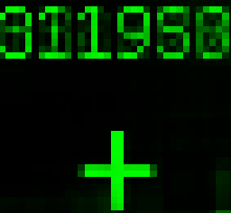
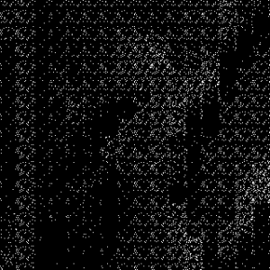
Here is an example SDR created from an image by sampling it in blocks (convolution where the stride equals the size of the receptive field):
Here is a convolutional reconstruction of the image, with a stride of 4 (I got impatient 🙂 ):

And finally, I leave you with an animated gif of the formation of the receptive fields over time:

Until next time!