Hello,
It’s been a while since I have posted here again, but I have been working on my CHTM reinforcement learner all along! I got it to perform pole balancing based on vision data of the pole alone recently, but only for a few seconds at a time. But that is a topic for another post. In this post, I want to discuss the changes and improvements that have occurred in CHTM – land.
For those unfamiliar, CHTM (continuous hierarchical temporal memory) is a generalization/simplification of the standard HTM developed by Numenta that uses familiar concepts from deep learning to reproduce the spatial pooling and temporal inference capabilities of standard HTM. The main change is that instead of using binary values for everything, we now use real-valued numbers for everything. This makes it simpler to code, and also provides some extra capabilities that the original did not have.
First let’s lay down the data structures we will be using in pseudocode.
struct Layer {
    Column[] columns;
};

struct Column {
    float activation;
    float state;
    float usage;

    Cell[] cells;

    Connection[] feedforwardConnections;
};

struct Cell {
    float prediction;
    float state;

    Connection[] lateralConnections;
};

struct Connection {
    float weight;
    float trace;

    int sourceIndex;
};
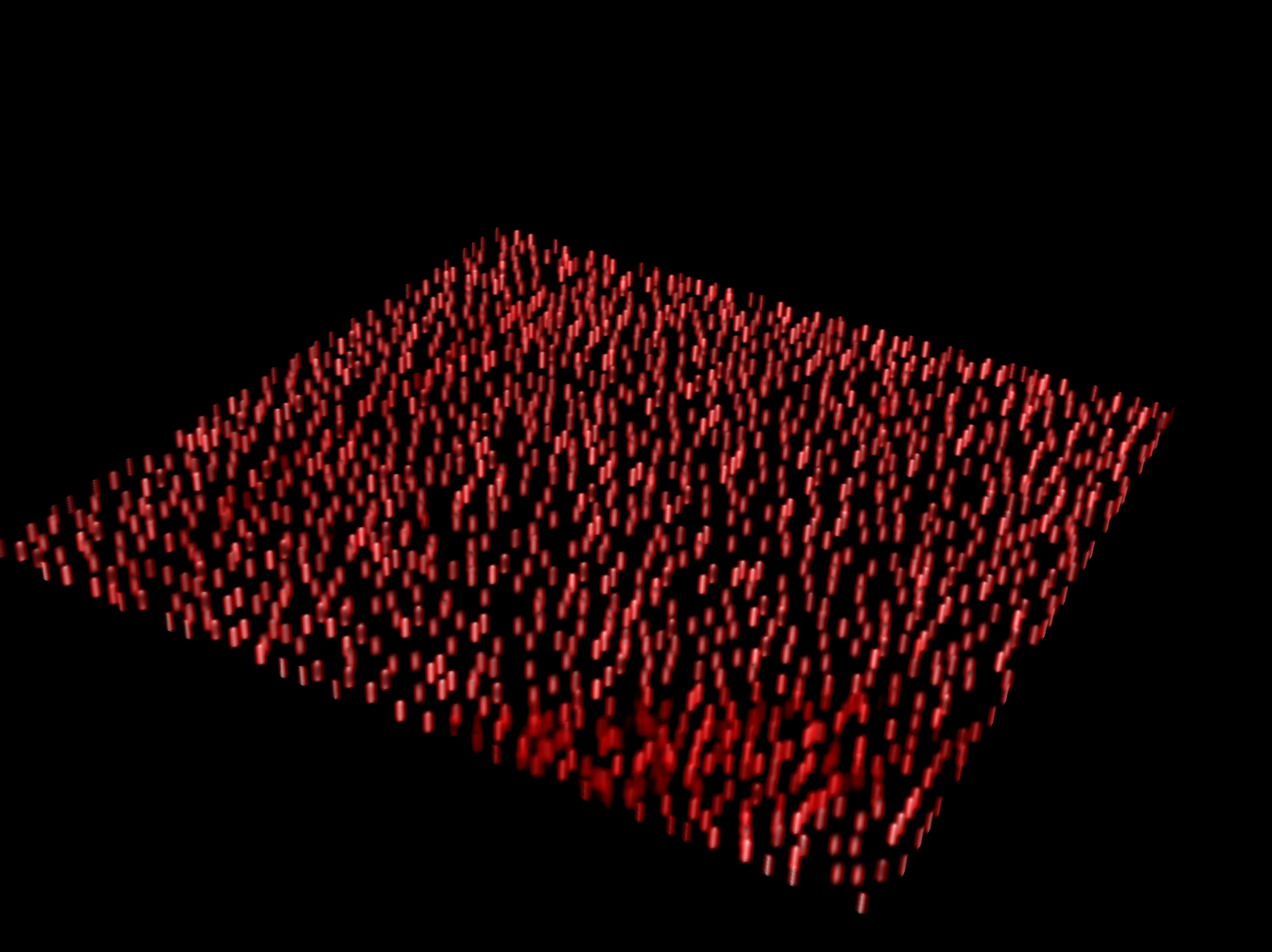
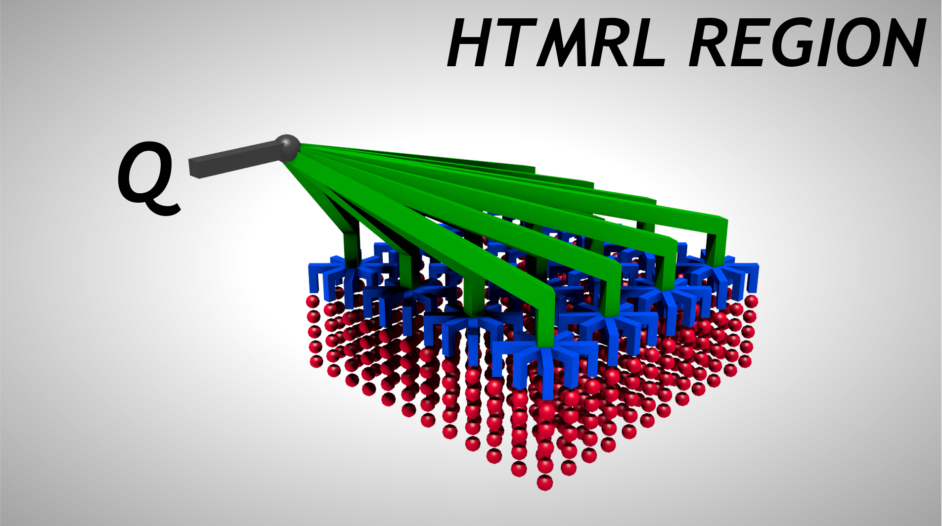
A layer consists of a 2D grid of columns. Each column has feedforward connections to an input source, taking a subsection of the input source (within a radius of the column). Each column also has a number of cells in it, which have lateral connections to other cells in the same layer within a radius.
CHTM, like the original, has two parts to it: Spatial pooling and temporal inference. Let’s start with spatial pooling. I will use the notation _(t-1) to describe values from a previous timestep.
In spatial pooling, when want to learn sparse distributed representations of the input such that the representations have minimal overlap. To do this, we go through each column (possibly in parallel) and calculate the activation value of each column:
void calculateActivations(Layer l, float[] input) {
foreach (Column col in l.columns) {
float sum = 0;
foreach (Connection con in col.feedforwardConnections) {
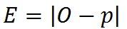
float difference = con.weight - input[con.sourceIndex];
sum += difference * difference;
}
col.activation = -sum;
}
}
Essentially what we are doing here is getting the negative distance between the input region and the feedforward connections vector. So the closer the column’s feedforward connections are to the input, the higher its activation value will be, capping out at 0.
The next step is the inhibition step:
void inhibit(Layer l, Radius inhibitionRadius, float localActivity, float stateIntensity, float usageDecay) {
foreach (Column col in l.columns) {
int numHigher = 0;
foreach (Column competitor in inhibitionRadius) {
if (competitor.activation > col.activation)
numHigher++;
}
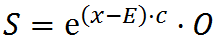
col.state = sigmoid((localActivity - numHigher) * stateIntensity);
col.usage = (1 - usageDecay) * (1 - col.state) * col.usage + col.state;
}
}
Here column states are set such that they are a sparsified version of the activation values. Along with that we update a usage parameter, which is a value that goes to 1 when a column’s state is 1 and decays when it is below 1. This way we can keep track of which columns are underutilized.
Next comes the learning portion of the spatial pooler:
void learnColumns(Layer l, float learningRate, float boostThreshold) {
foreach (Column col in l.columns) {
float learnScalar = learningRate * min(1, max(0, boostThreshold - col.usage) / boostThreshold);
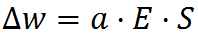
foreach (Connection con in col.feedforwardConnections)
con.weight += learnScalar * (input[con.sourceIndex] - con.weight);
}
}
Here we move underutilized columns towards the current input vector. This way we maximize the amount of information the columns can represent.
Next up: The temporal inference component!

 of a neuron to its inputs